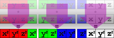
Recently, I wanted to see how fast I could make a function that normalizes every vector in an array. The goal was to take “natural” data and make it as fast as possible without putting any undue restrictions on the caller, such as alignment. While this article specifically uses 128 bit SSE vectors comprised of four floats, the same general concept applies to any size vector on any platform.
While I do cover some of the basics of what SIMD is, why it’s faster, etc., this is by no means meant to be a tutorial on the subject. If you’re looking for one, there are lots of them out there, try searching.
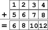
SIMD, or Single Instruction Multiple Data, is a way of having one instruction apply to multiple pieces of data. For example, if I have two SIMD vectors and I add them together, it’s one instruction (ADDPS, for example) that applies to every element of each of the vectors:

When done with scalar math, each addition is a single instruction, so theoretically you could run at 4x speed if you have perfect scalar to SIMD math conversions. Of course, it never works out this way, but that’s a topic for another discussion…
Vector math libraries typically come in one of two varieties: a 3 element { x, y, z } or a 4 element { x, y, z, w } version. Since the w component of a 4 element vector is usually 1 for a point or 0 for a vector, it’s typically left off. Keeping it can cost a fairly significant amount of memory and the usage (point versus ray) can be assumed in most uses.
Here’s a SIMD vector4 in memory:

Here’s a scalar vector3 in memory:

The colored block [–] marks 16 byte boundaries. CPUs are really good at loading aligned data and SIMD vectors always start with X on an even 16 byte boundary, making them really fast. The scalar version aligns on a natural boundary of a float, or 4 bytes. Not being on an even 16 byte boundary, it is very slow to get into or out of SIMD.
Here’s our scalar vec3 definition:
<pre>typedef struct _vec3
{
  float x;
  float y;
  float z;
} vec3;</pre>
Here’s a function to normalize a single vector:
inline void vec3Normalize(const vec3 * const in, vec3 * const out)
{
  const float len = sqrt(in->x * in->x + in->y * in->y + in->z * in->z);
  out->x = in->x / len;
  out->y = in->y / len;
  out->z = in->z / len;
}
And here’s our naïve method of a scalar batch normalize:
void vec3BatchNormalize(const vec3 * const in,
                        const uint32_t count,
                        vec3 * const out)
{
  for (uint32_t i = 0; i < count; ++i)
  {
    vec3Normalize(&in[i], &out[i];
  }
}
We could convert this code to SIMD by loading the vec3’s into SIMD registers, but we have a few problems. First, our data isn’t aligned, so it’s going to be slow. Second, you can’t load a vec3 into a SIMD vec4 without reading either the X component of the next vector or invalid memory.
To fix the first issue, we know that the input data will be on a natural alignment of 4 bytes. This means that a 16 byte aligned vector will be found in at most 4 vec3’s, or 12 floats. We’ll call this our “pre-pass” vectors, since these are the ones we’ll handle individually before the real batch processing begins.
To fix the second issue, we could just process the data differently. Rather than handling a single vector at a time, we can do four at a time. This also relates to alignment – if we process four at a time, we’re guaranteed to always be aligned. To determine how many we can do, the math is simply (count – prepass) & (~3). We’ll call this our “mid-pass” count.
Of course, we have to process the trailing vectors as well, but that’s simply whatever’s left over, or (count – (prepass + midpass)).
Before inserting SIMD, we have this code as a template to work with:
void vec3BatchNormalizeSSE0(const vec3 * const in,
                            const uint32_t count,
                            vec3 * const out)
{
  const uint32_t prepass  = ((uintptr_t)in & 0xf) / 4;
  const uint32_t midpass  = (count - prepass) & ~3;
  for (uint32_t i = 0; i < prepass; ++i)
  {
    vec3Normalize(&in[i], &out[i]);
  }
  for (uint32_t i = prepass; i < prepass + midpass; ++i)
  {
    vec3Normalize(&in[i], &out[i]);
  }
  for (uint32_t i = prepass + midpass; i < count; ++i)
  {
    vec3Normalize(&in[i], &out[i]);
  }
}
Processing the vectors four at a time makes things a bit more interesting. We start by loading four vec3’s into three vec4’s:
    const float * const src = &in[i].x;
    const __m128 source[] =
    {
      _mm_load_ps(src + 0),
      _mm_load_ps(src + 4),
      _mm_load_ps(src + 8)
    };
It looks like this in memory (I’ve colored the scalar vectors to make them easier to see):

To normalize a vector, we divide it by it’s length which is sqrt(x*x + y*y + z*z). So our first SIMD operation is (x*x + y*y + z*z) but there’s a problem: that’s a vec3 normal and our first vec4 is filled with { x, y, z, x } instead.
No worries! By processing them four at a time, we can make use of the w component to do some work for us as well. Rather than simply leaving the w component as zero or one, or worse, taking the time to zero it out, we use that slot for data in the next vector. We’re doing the same calculation later, so we may as well use the slot!
Multiply the vectors by themselves to get the squared values:
    const __m128 square[] =
    {
      _mm_mul_ps(source[0], source[0]),
      _mm_mul_ps(source[1], source[1]),
      _mm_mul_ps(source[2], source[2])
    };
In memory, the result of the multiply looks like this:

Using the shuffle instruction, we can move the vector around so we can sum the results in one pass. Because of our data organization, we have to do this in two steps:
    const __m128 xpose1[] =
    {
      _mm_shuffle_ps(square[0], square[1], _MM_SHUFFLE(1, 0, 1, 0)),
      _mm_shuffle_ps(square[1], square[2], _MM_SHUFFLE(3, 2, 3, 2)),
      _mm_shuffle_ps(square[0], square[2], _MM_SHUFFLE(1, 0, 3, 2))
    };
    const __m128 xpose2[] =
    {
      _mm_shuffle_ps(xpose1[0], xpose1[2], _MM_SHUFFLE(3, 2, 2, 0)),
      _mm_shuffle_ps(xpose1[0], xpose1[1], _MM_SHUFFLE(3, 1, 3, 1)),
      _mm_shuffle_ps(xpose1[2], xpose1[1], _MM_SHUFFLE(2, 0, 1, 0))
    };
Now we can easily sum all three of the vectors into one final squared length vector and calculate the reciprocal square root:
    const __m128 sum1 = _mm_add_ps(xpose2[1], xpose2[2]);
    const __m128 lensq = _mm_add_ps(xpose2[0], sum1);
    const __m128 rcpsqrt = _mm_rsqrt_ps(lensq);
We now have a vector that contains the scale for the original data, but is, yet again, out of order. To fix it, we reshuffle the resulting vector out to three vectors that we can multiply against the original input:
    const __m128 scale[] =
    {
      _mm_shuffle_ps(rcpsqrt, rcpsqrt, _MM_SHUFFLE(1, 0, 0, 0)),
      _mm_shuffle_ps(rcpsqrt, rcpsqrt, _MM_SHUFFLE(2, 2, 1, 1)),
      _mm_shuffle_ps(rcpsqrt, rcpsqrt, _MM_SHUFFLE(3, 3, 3, 2))
    };
Multiply the original input vectors by the scale, creating the normal vectors:
    const __m128 norm[] =
    {
      _mm_mul_ps(source[0], scale[0]),
      _mm_mul_ps(source[1], scale[1]),
      _mm_mul_ps(source[2], scale[2])
    };
And, finally, store the normals to the output buffer. Since we don’t know the alignment of the output, we have to do unaligned stores, which are very slow:
    float * const dst = &out[i].x;
    _mm_storeu_ps(dst + 0, norm[0]);
    _mm_storeu_ps(dst + 4, norm[1]);
    _mm_storeu_ps(dst + 8, norm[2]);
Here’s the full code, ready for your copy/paste pleasure:
void vec3BatchNormalizeSSE1(const vec3 * const in,
                            const uint32_t count,
                            vec3 * const out)
{
  const uint32_t prepass = ((uintptr_t)in & 0xf) / 4;
  const uint32_t midpass = (count - prepass) & ~3;
  // process as many vectors as it takes to get to aligned data
  for (uint32_t i = 0; i < prepass; ++i)
  {
    vec3Normalize(&in[i], &out[i]);
  }
  for (uint32_t i = prepass; i < prepass + midpass; i += 4)
  {
    // load the vectors from the source data
    const float * const src = &in[i].x;
    const __m128 source[] =
    {
      _mm_load_ps(src + 0),
      _mm_load_ps(src + 4),
      _mm_load_ps(src + 8)
    };
    // compute the square of each vector
    const __m128 square[] =
    {
      _mm_mul_ps(source[0], source[0]),
      _mm_mul_ps(source[1], source[1]),
      _mm_mul_ps(source[2], source[2])
    };
    // prepare to add, transposing the data into place
    // first transpose
    //
    // x0, y0, z0, x1    x0, y0, y1, z1
    // y1, z1, x2, y2 => x2, y2, y3, z3
    // z2, x3, y3, z3    z0, x1, z2, x3
    const __m128 xpose1[] =
    {
      _mm_shuffle_ps(square[0], square[1], _MM_SHUFFLE(1, 0, 1, 0)),
      _mm_shuffle_ps(square[1], square[2], _MM_SHUFFLE(3, 2, 3, 2)),
      _mm_shuffle_ps(square[0], square[2], _MM_SHUFFLE(1, 0, 3, 2))
    };
    // second transpose
    //
    // x0, y0, y1, z1    x0, y1, z2, x3
    // x2, y2, y3, z3 => y0, z1, y2, z3
    // z0, x1, z2, x3    z0, x1, x2, y3
    const __m128 xpose2[] =
    {
      _mm_shuffle_ps(xpose1[0], xpose1[2], _MM_SHUFFLE(3, 2, 2, 0)),
      _mm_shuffle_ps(xpose1[0], xpose1[1], _MM_SHUFFLE(3, 1, 3, 1)),
      _mm_shuffle_ps(xpose1[2], xpose1[1], _MM_SHUFFLE(2, 0, 1, 0))
    };
    // sum the components to get the squared length
    const __m128 sum1 = _mm_add_ps(xpose2[1], xpose2[2]);
    const __m128 lensq = _mm_add_ps(xpose2[0], sum1);
    // calculate the scale as a reciprocal sqrt
    const __m128 rcpsqrt = _mm_rsqrt_ps(lensq);
    // to apply it, we have to mangle it around again
    //               s0, s0, s0, s1
    // x, y, z, w => s1, s1, s2, s2
    //               s2, s3, s3, s3
    const __m128 scale[] =
    {
      _mm_shuffle_ps(rcpsqrt, rcpsqrt, _MM_SHUFFLE(1, 0, 0, 0)),
      _mm_shuffle_ps(rcpsqrt, rcpsqrt, _MM_SHUFFLE(2, 2, 1, 1)),
      _mm_shuffle_ps(rcpsqrt, rcpsqrt, _MM_SHUFFLE(3, 3, 3, 2))
    };
    // multiply the original vector by the scale, completing the normalize
    const __m128 norm[] =
    {
      _mm_mul_ps(source[0], scale[0]),
      _mm_mul_ps(source[1], scale[1]),
      _mm_mul_ps(source[2], scale[2])
    };
    // store the result into the output array (unaligned data)
    float * const dst = &out[i].x;
    _mm_storeu_ps(dst + 0, norm[0]);
    _mm_storeu_ps(dst + 4, norm[1]);
    _mm_storeu_ps(dst + 8, norm[2]);
  }
  // process any leftover vectors indivually
  for (uint32_t i = prepass + midpass; i < count; ++i)
  {
    vec3Normalize(&in[i], &out[i]);
  }
}
As a first pass, that’s a pretty significant improvement. My perf testing in release (MS Visual Studio in /O2) reports these clock cycles per batch normalize (10,000 runs with 1,000 warm-up passes of 4107 pre-generated vec3’s):
                Name:       Total    Shortest     Longest     Average
              scalar   7,278,466          658     180,093         659
       first attempt   1,312,945          117     112,395         117
That’s not too shabby of a start! The SIMD version runs in about 18% of the total time of the original.
In fact, here’s the same run with /Ox optimizations turned on with the SIMD version running in about 19% of the scalar time:
                Name:       Total    Shortest     Longest     Average
              scalar   7,532,213          658     246,995         659
       first attempt   1,429,562          117     112,923         117
And just to cover some more bases, here’s the debug run with optimizations disabled, running in about 34% of the scalar time:
                Name:       Total    Shortest     Longest     Average
              scalar  16,559,810         1530     273,216        1530
       first attempt   5,659,434          520      95,957         520
Here’s where it gets really fun, though. The above version is somewhat naïve in that it doesn’t take into account data loads, pipelining, etc. The only pipelining being done is by the compiler and the CPU at runtime. We can definitely do better.
But that’s for the next post!